Analyzing and Interpreting Speech Patterns from a Sound File with Praat and Parselmouth

Introduction

Praat is a popular software package mainly used for speech analysis. It has been around since 1995 and is still widely used in linguistics and NLP fields. While being consistently updated by its creators Paul Boersma and David Weenink of the University of Amsterdam, its website is a mid-90s time capsule. Praat has a broad functionality, and supports spectrogram visualization, pitch tracking, formant analysis, and speech synthesis.

Parselmouth is a Python library built specifically to interact with Praat and audio files, creating a seamless development environment to utilize the power of Python and Praat. The goal of Parselmouth is specifically to provide a “Pythonic” interface to Praat, rather than using the native C-based script that the software uses.

In this tutorial I hope to give you a very brief look into the capabilities of Praat, and some strategies to use Parselmouth for NLP tasks.

Requirements

In order to run the examples in this tutorial, you will need Python 3 or higher, Praat Version 6.03.09, and the Parsertongue Python Library installed on your machine. These were run within Jupyter notebooks in a native Linux environment (Ubuntu 20.04.6). All supplemental software referenced here is licensed under the GNU General Public License V3, and is open source.

Loading a Sound file Using Parselmouth

Parselmouth makes it very easy to load a sound file for analysis.

import parselmouth as pm

sound = pm.Sound(Test.wav) 

From there, the file is ready to be read and manipulated using Praat.

The included test file includes a short clip of me saying “This is a sentence I am recording for Praat.” Feel free to use any audio file you’d like, but know that these programs are happiest when working with .wav files.

Here is an example of a variable made using Parselmouth’s pitch method, which stores information about the pitch over the duration of the audio file.

pitch = sound.to_pitch()
print(pitch)

Object type: Pitch
Object name: <no name>
Date: Sat May  6 13:22:20 2023

Time domain:
   Start time: 0 seconds
   End time: 2.72115625 seconds
   Total duration: 2.72115625 seconds
Time sampling:
   Number of frames: 269 (189 voiced)
   Time step: 0.01 seconds
   First frame centred at: 0.020578125 seconds
Ceiling at: 600 Hz

Estimated quantiles:
   10% = 83.4895308 Hz = 77.7288574 Mel = -3.12399353 semitones above 100 Hz = 2.56696611 ERB
   16% = 84.669073 Hz = 78.751992 Mel = -2.88111601 semitones above 100 Hz = 2.59933851 ERB
   50% = 96.1593296 Hz = 88.6203095 Mel = -0.67801508 semitones above 100 Hz = 2.90961122 ERB
   84% = 503.023015 Hz = 357.22615 Mel = 27.9674929 semitones above 100 Hz = 10.3309131 ERB
   90% = 549.888459 Hz = 381.175176 Mel = 29.5096681 semitones above 100 Hz = 10.920997 ERB
Estimated spreading:
   84%-median = 407.9 Hz = 269.3 Mel = 28.72 semitones = 7.441 ERB
   median-16% = 11.52 Hz = 9.895 Mel = 2.209 semitones = 0.3111 ERB
   90%-10% = 467.6 Hz = 304.3 Mel = 32.72 semitones = 8.376 ERB

Minimum 75.236856 Hz = 70.5167481 Mel = -4.92586238 semitones above 100 Hz = 2.33766131 ERB
Maximum 592.814486 Hz = 402.232088 Mel = 30.8109684 semitones above 100 Hz = 11.4324657 ERB
Range 517.6 Hz = 331.715339 Mel = 35.74 semitones = 9.095 ERB
Average: 214.312673 Hz = 165.69488 Mel = 7.19169562 semitones above 100 Hz = 5.02663409 ERB
Standard deviation: 191.9 Hz = 125.9 Mel = 13.61 semitones = 3.478 ERB

Mean absolute slope: 2470 Hz/s = 1580 Mel/s = 170.6 semitones/s = 43.31 ERB/s
Mean absolute slope without octave jumps: 51.9 semitones/s

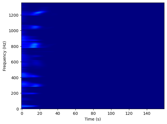
Simple plots Using Matplotlib

We can use other common libraries like Matplotlib to visualize the recording, with things like spectrograms:

import parselmouth
import matplotlib.pyplot as plt

voice = parselmouth.Sound("Test.wav")

spectrogram = voice.to_spectrogram()

plt.imshow(spectrogram.values.T, aspect='auto', origin='lower', cmap='jet')
plt.xlabel("Time (s)")
plt.ylabel("Frequency (Hz)")
plt.show()

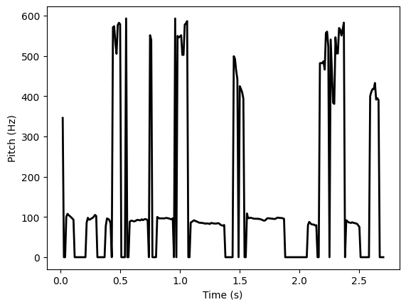
…or pitch contour plots:

pitch = voice.to_pitch()

# Get the pitch contour values and times
pitch_values = pitch.selected_array['frequency']
pitch_times = pitch.xs()

plt.plot(pitch_times, pitch_values, linewidth=2, color='black')
plt.xlabel("Time (s)")
plt.ylabel("Pitch (Hz)")
plt.show()

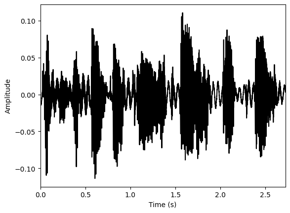
…or simple waveform displays:

waveform = sound.values.T

duration = sound.duration

time = sound.xmin + np.arange(len(waveform)) / float(sound.sampling_frequency)

plt.plot(time, waveform, color='black')
plt.xlabel('Time (s)')
plt.ylabel('Amplitude')
plt.xlim([0, duration])
plt.show()

We can also average measurements like pitch and formants across the span of a sound file.

import numpy as np
pitch_values = pitch.selected_array['frequency']
mean_pitch = np.mean(pitch_values)

print(mean_pitch)

150.57656235439302

While averaging an entire sentence may not be very useful, averaging many individual waveform files split into single words or phonemes can be used as features for classifying the demographics of the speaker. The resulting values can be used for recognizing speech emotion, the identity of the speaker, or even regional accents.

Displaying Formant Data as an Array

Here’s a simple function to display formant data (visualized above) for three formants at all of the key times stored in the formants object.

import parselmouth
import numpy as np

def display_formants(file_path):

    """
    Displays formants as F1, F2, and F3 at certain increments of time from an audio file.
    Input:  A file path
    Output: Prints an array of formants at increments of time
    """
    sound = parselmouth.Sound(file_path)

    formants = sound.to_formant_burg(max_number_of_formants=3)

    times = formants.xs()
    formant_values = np.array([[
    formants.get_value_at_time(1, t), 
    formants.get_value_at_time(2, t), 
    formants.get_value_at_time(3, t) 
    ] for t in times])

    print("Formant values:")
    for t, f1, f2, f3 in zip(times, formant_values[:,0], formant_values[:,1], formant_values[:,2]):
        print("Time: {:.3f}, F1: {:.2f}, F2: {:.2f}, F3: {:.2f}".format(t, f1, f2, f3))

display_formants("Test.wav")

#Only the first 20 results shown
Formant values:
Time: 0.026, F1: 679.66, F2: 3871.67, F3: nan
Time: 0.032, F1: 591.46, F2: 2979.99, F3: 4231.13
Time: 0.039, F1: 494.59, F2: 3985.75, F3: nan
Time: 0.045, F1: 315.03, F2: 3583.33, F3: nan
Time: 0.051, F1: 316.56, F2: 2808.21, F3: 3915.48
Time: 0.057, F1: 339.82, F2: 2265.67, F3: 3843.62
Time: 0.064, F1: 368.22, F2: 2277.89, F3: 3825.53
Time: 0.070, F1: 386.27, F2: 2365.04, F3: 3839.37
Time: 0.076, F1: 389.71, F2: 2527.27, F3: 3900.74
Time: 0.082, F1: 390.98, F2: 2522.16, F3: 3947.92
Time: 0.089, F1: 402.59, F2: 2296.24, F3: 3923.87
Time: 0.095, F1: 406.99, F2: 2533.48, F3: 4143.36
Time: 0.101, F1: 367.42, F2: 2896.31, F3: 4414.31
Time: 0.107, F1: 3353.61, F2: 4466.30, F3: nan
Time: 0.114, F1: 102.56, F2: 3563.72, F3: 4559.57
Time: 0.120, F1: 3783.21, F2: 4607.31, F3: nan
Time: 0.126, F1: 3855.56, F2: 4653.59, F3: nan
Time: 0.132, F1: 3873.59, F2: 4685.67, F3: nan
Time: 0.139, F1: 4538.29, F2: 4726.09, F3: nan
Time: 0.145, F1: 536.70, F2: 4211.27, F3: 4690.90
Time: 0.151, F1: 3807.91, F2: 4717.06, F3: nan
Time: 0.157, F1: 3710.77, F2: 4772.50, F3: nan
Time: 0.164, F1: 3874.92, F2: 4871.99, F3: nan
Time: 0.170, F1: 198.48, F2: 3923.39, F3: 4749.48
Time: 0.176, F1: 586.72, F2: 4175.50, F3: 4601.51
Time: 0.182, F1: 3976.58, F2: 4574.92, F3: nan
Time: 0.189, F1: 4000.93, F2: 4512.30, F3: nan
Time: 0.195, F1: 289.53, F2: 4279.48, F3: nan
Time: 0.201, F1: 509.61, F2: 3903.61, F3: 4920.06
Time: 0.207, F1: 3971.57, F2: 4813.88, F3: nan
Time: 0.214, F1: 237.33, F2: 3865.56, F3: 4607.74

Note that it is normal for formant calculations to include nan values, based on low input volume or noise.

From here, you could build prediction models for vowel or word prediction, or use silence data to split the .wav file up into individual phonemes, words, or phrases.